Question 3:
(b) Based on the completed table above,
Solution:
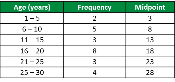
(a)
(b)(i)
(b)(ii)
(c)
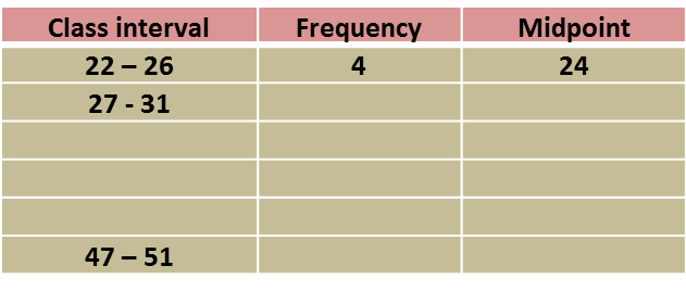
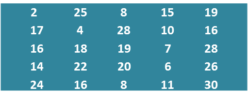
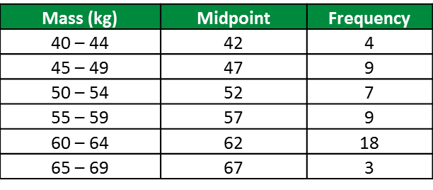
The data below shows the mass, in kg, of 50 students.
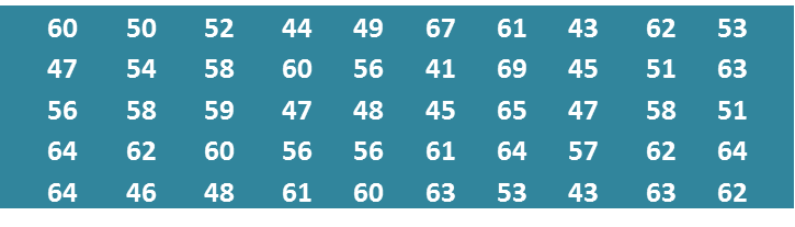
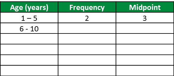
(a) Copy and complete the table below based on the data above.
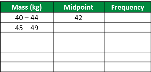
(a) Copy and complete the table below based on the data above.
(b) Based on the completed table above,
(i) State the size of the class interval used in the table.
(ii) Calculate the estimated mean of the mass of the students.
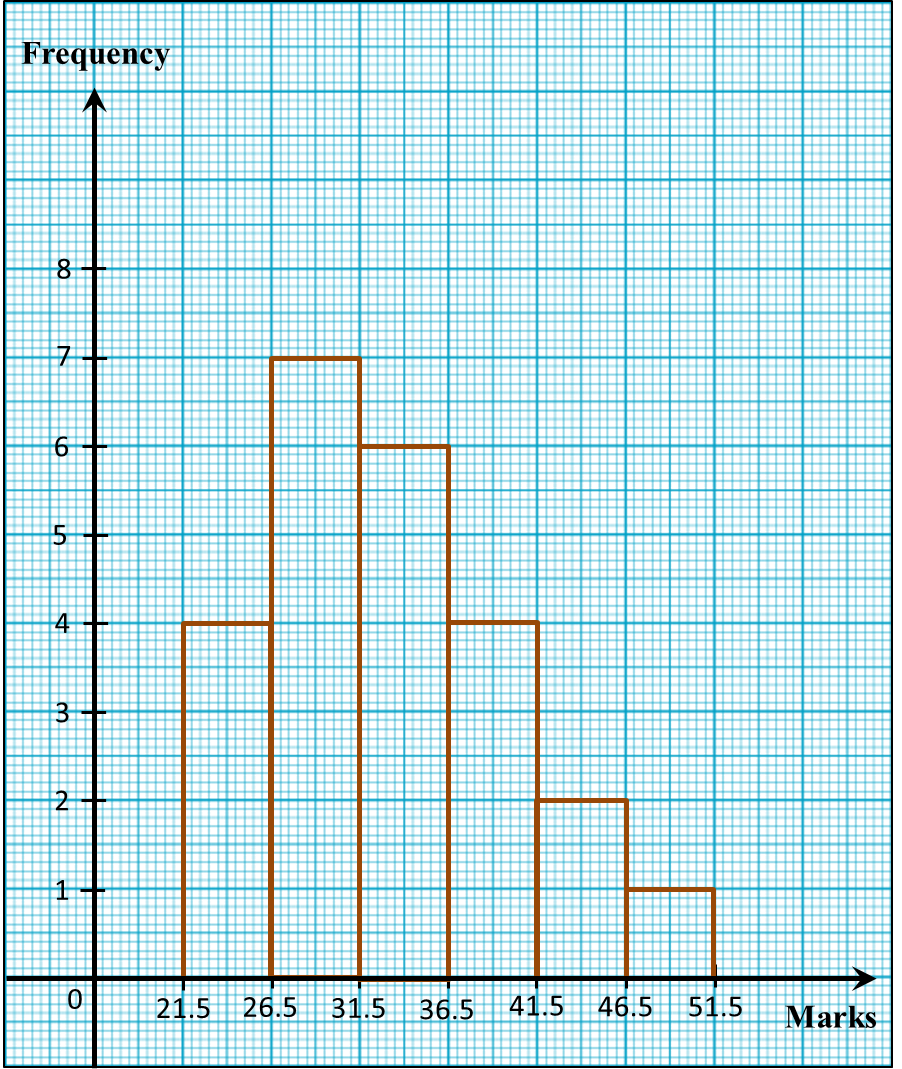
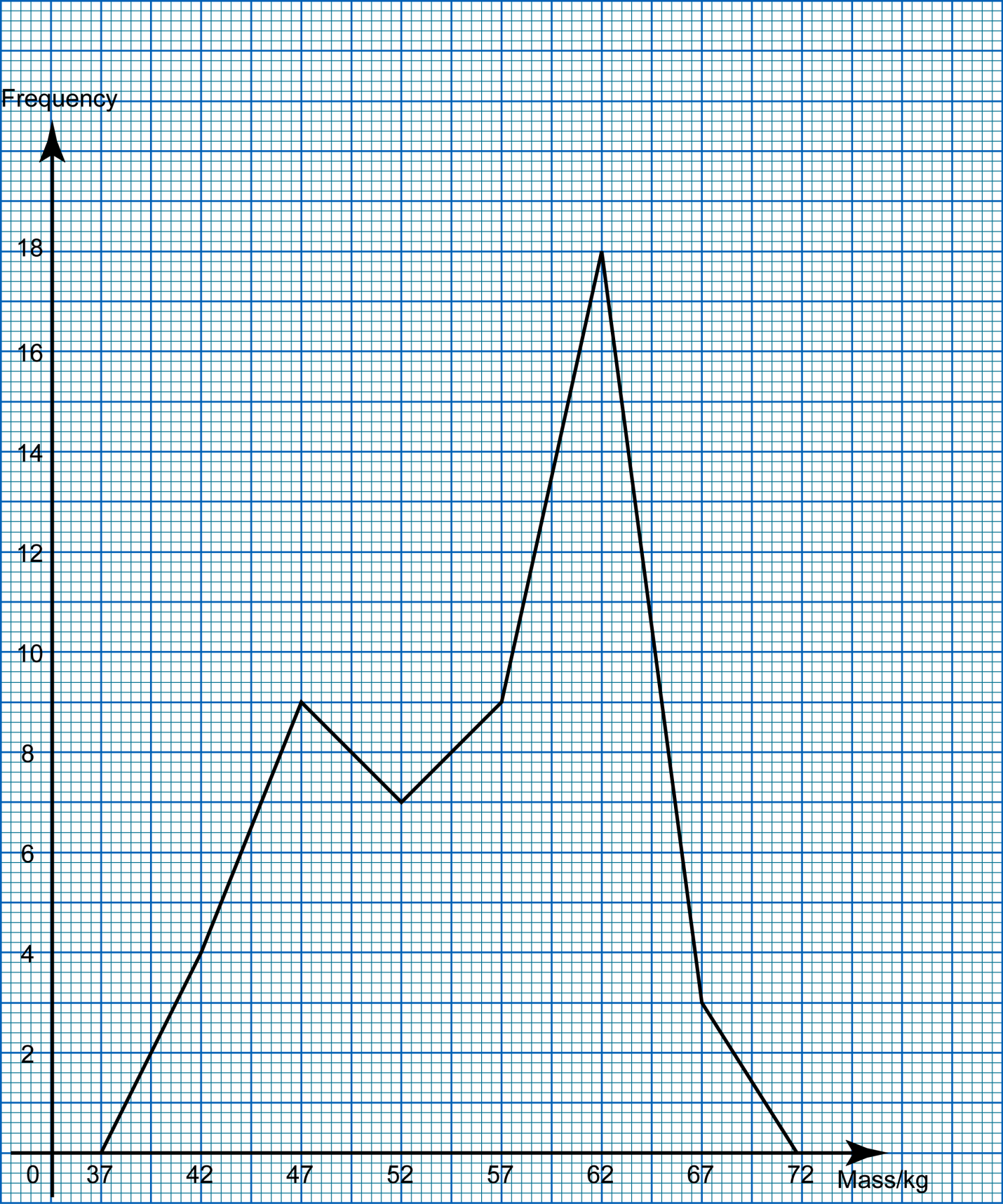
For this part of the question, use graph paper.
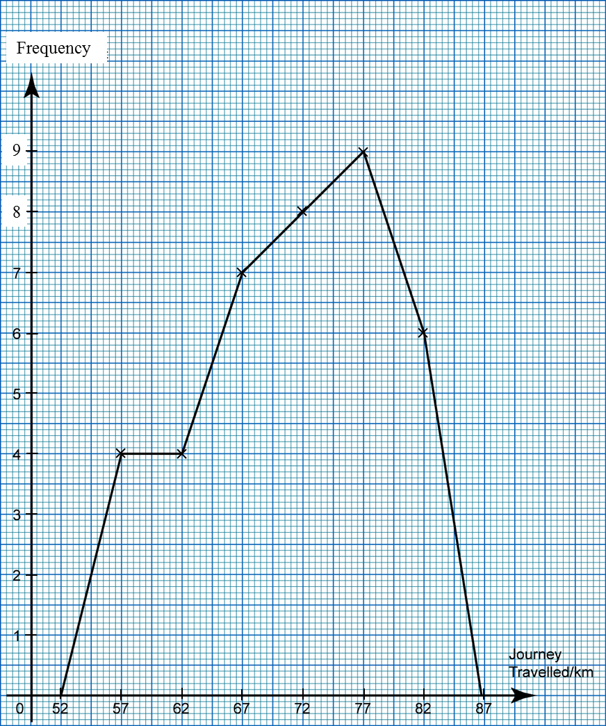
(c) By using a scale of 2 cm to 5 kg on the horizontal axis and 2 cm to 2 students on the vertical axis, draw a frequency polygon for the data.
For this part of the question, use graph paper.
(c) By using a scale of 2 cm to 5 kg on the horizontal axis and 2 cm to 2 students on the vertical axis, draw a frequency polygon for the data.
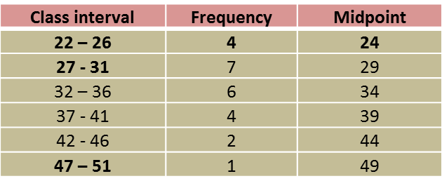
(a)
(b)(i)
Size of class interval
= upper boundary – lower boundary
= 44.5 – 39.5
= 5
(b)(ii)
(c)
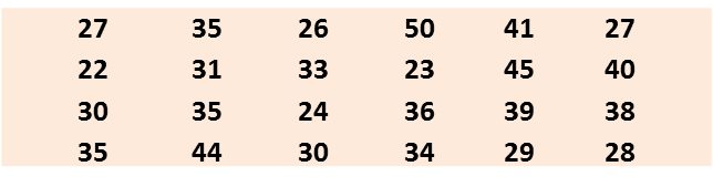 (a) Based on the data in diagram above, complete Table in the answer space.