Question 1:
(b) Based on the completed table above,
Solution:
(a)
Calculation of midpoint for (age 6 – 10) =
(b)(i)
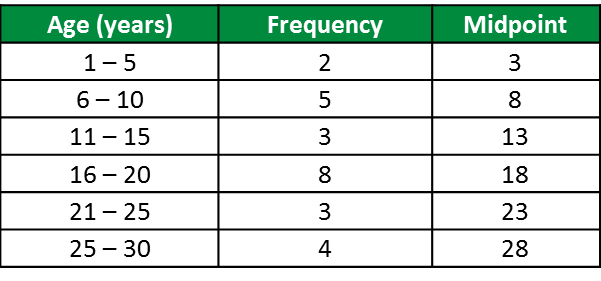
Modal class = age 16 – 20 (highest frequency)
(b)(ii)
(c)

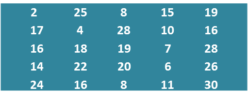
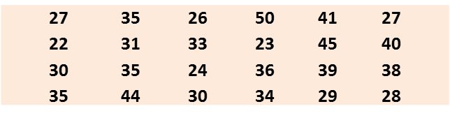
The data below shows the age of 25 tourists who visited a tourist spot.
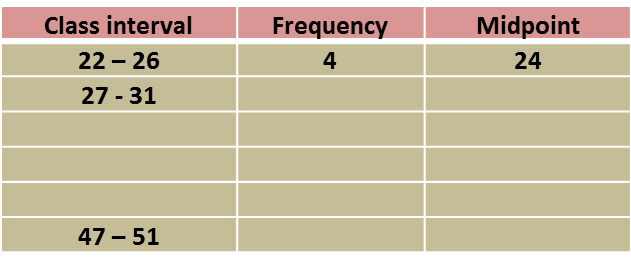
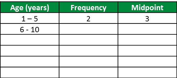
(a) Copy and complete the table below based on the data above.
(a) Copy and complete the table below based on the data above.
(b) Based on the completed table above,
(i) State the modal class.
(ii) Calculate the mean age of the tourists.
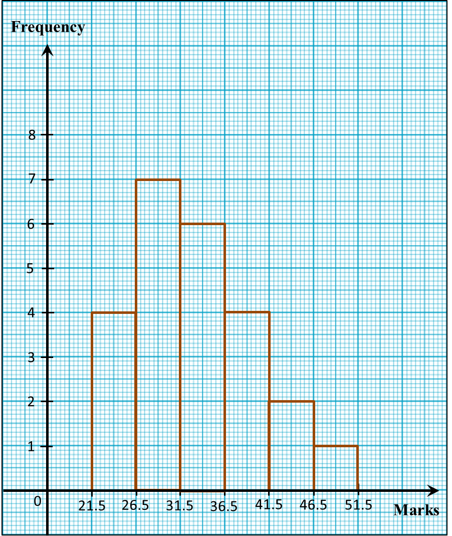
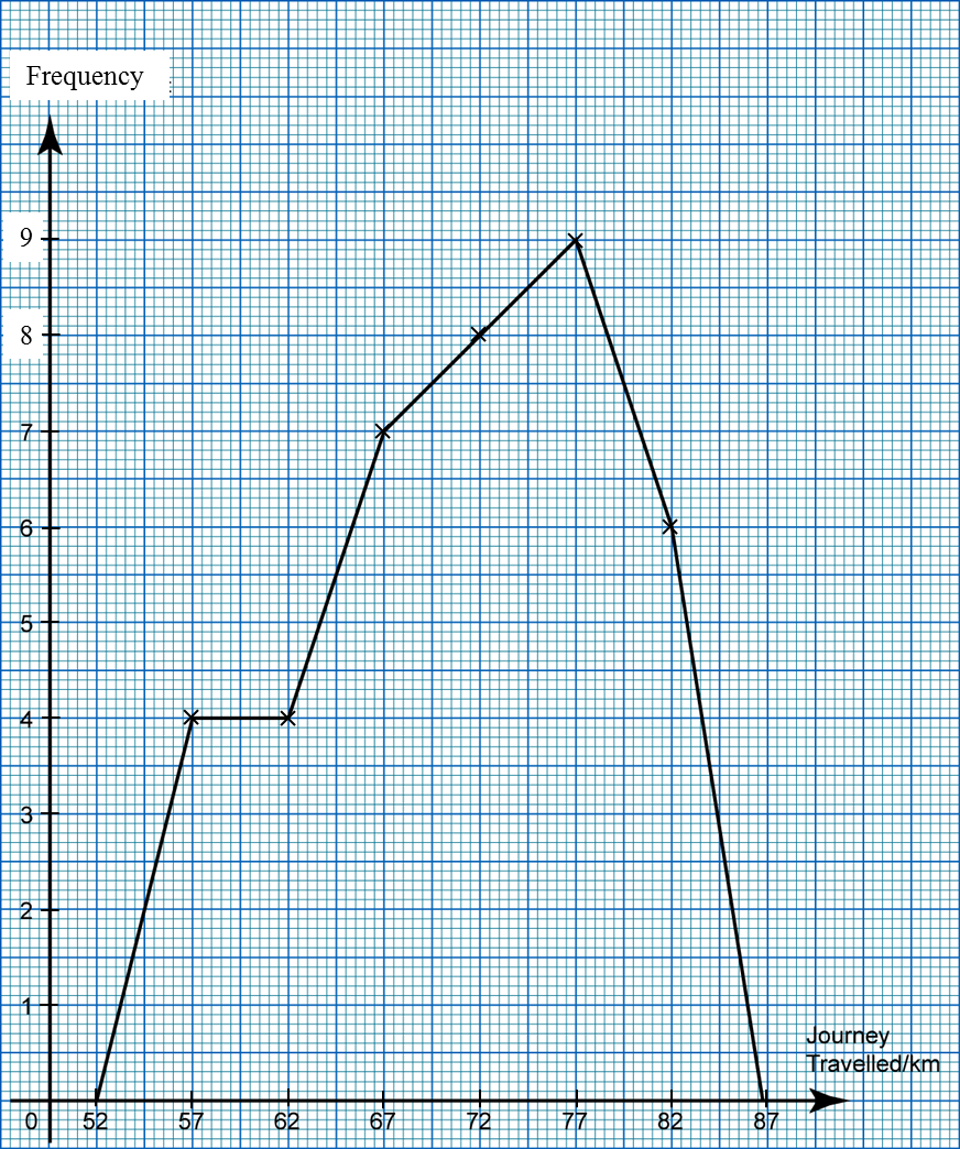
(c) For this part of the question, use graph paper.
(c) For this part of the question, use graph paper.
By using a scale of 2 cm to 5 years on the horizontal axis and 2 cm to 1 tourist on the vertical axis, draw a histogram for the data.
Solution:
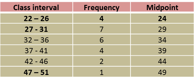
(a)
Calculation of midpoint for (age 6 – 10) =
(b)(i)
Modal class = age 16 – 20 (highest frequency)
(b)(ii)
(c)
 (a) Based on the data in diagram above, complete Table in the answer space.