Question 10 (12 marks):
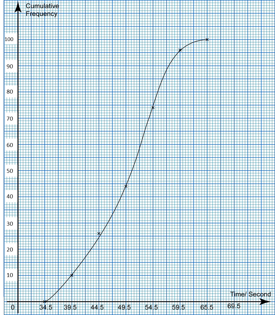
Diagram shows a histogram which represents the mass, in kg, for a group of 100 students.
 Diagram
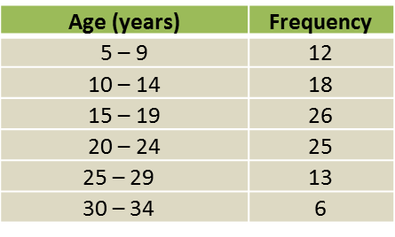
(a) Based on the Diagram, complete the Table in the answer space.
(b) Calculate the estimated mean mass of a student.
(c) For this part of the question, use graph paper. You may use a flexible curve ruler.
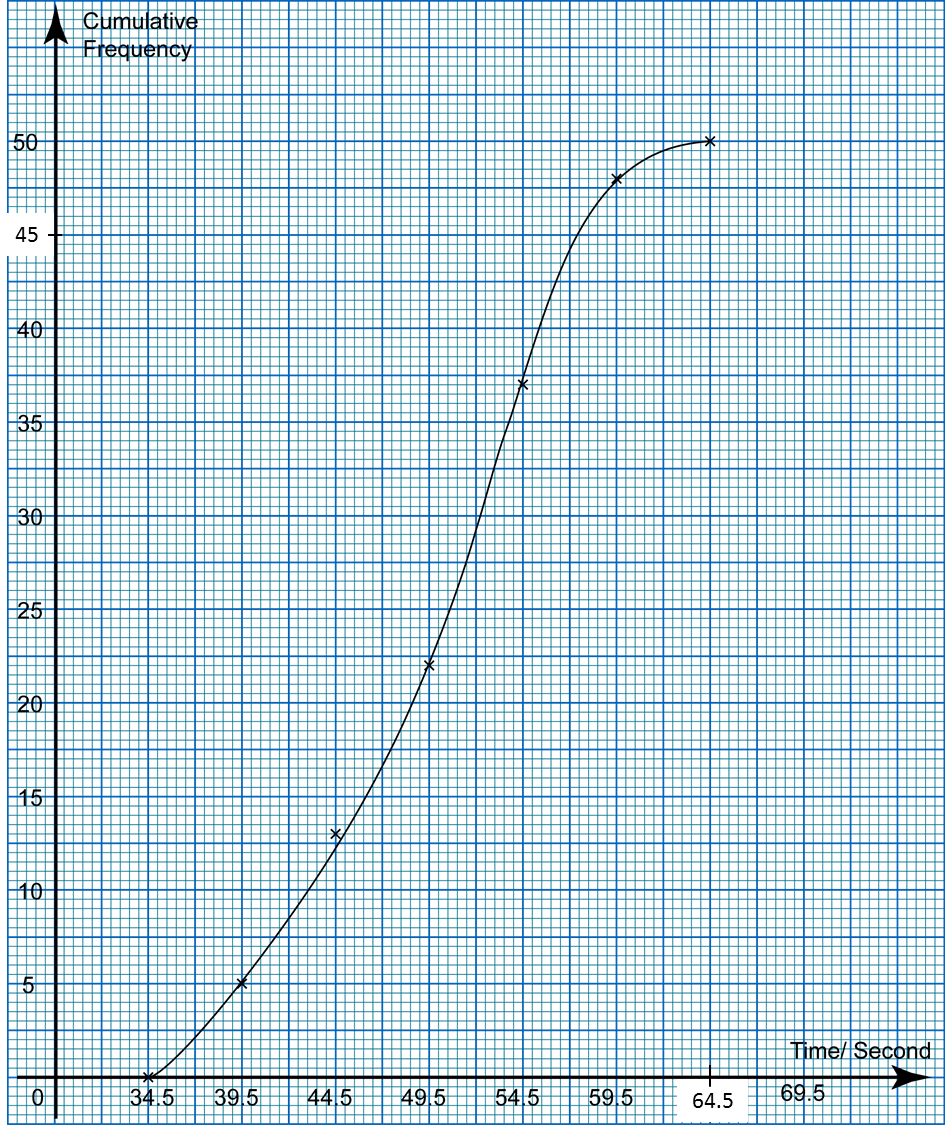
Using a scale of 2 cm to 10 kg on the horizontal axis and 2 cm to 10 students on the vertical axis, draw an ogive for the data.
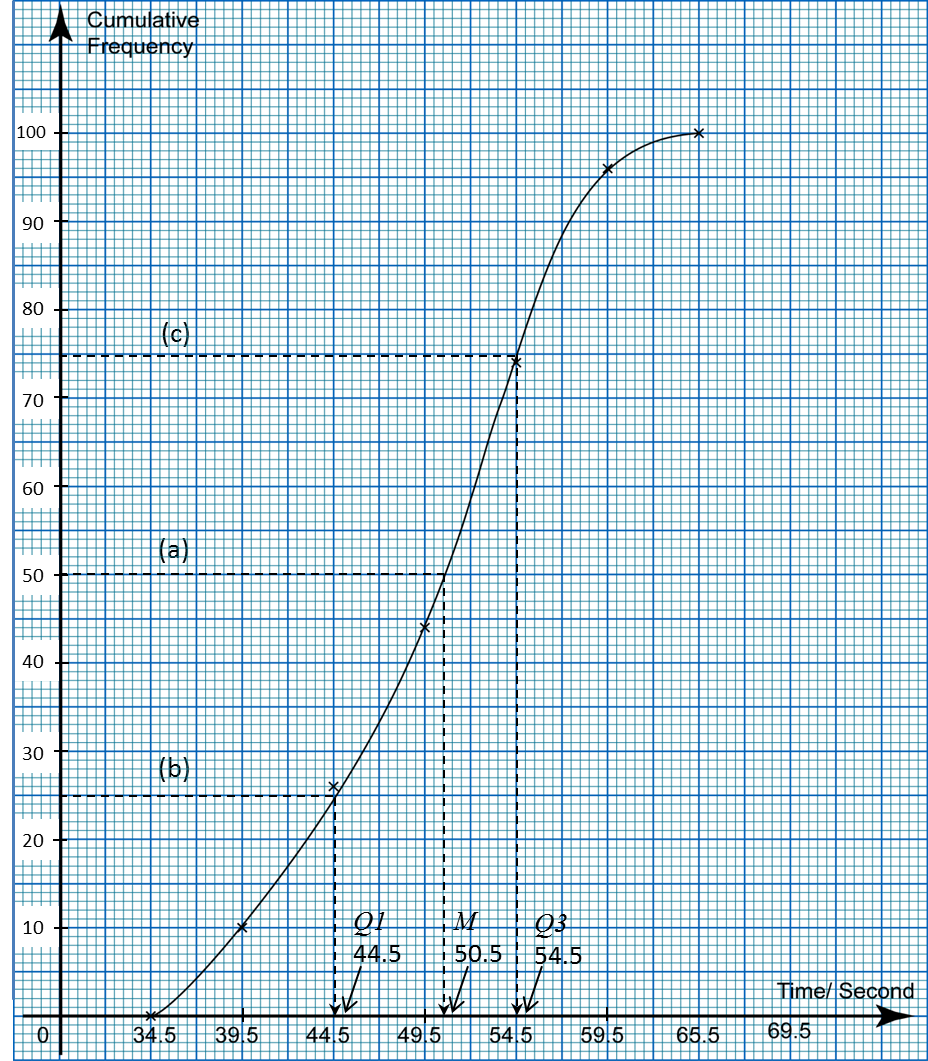
(d) Based on the ogive drawn in 10(c), state the third quartile.
Answer:

Solution:
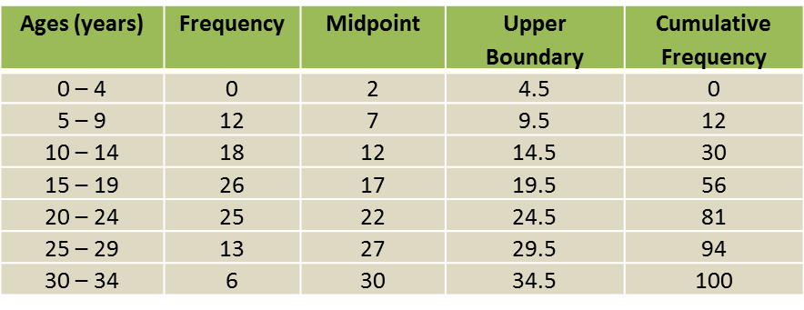
(a)

(b)

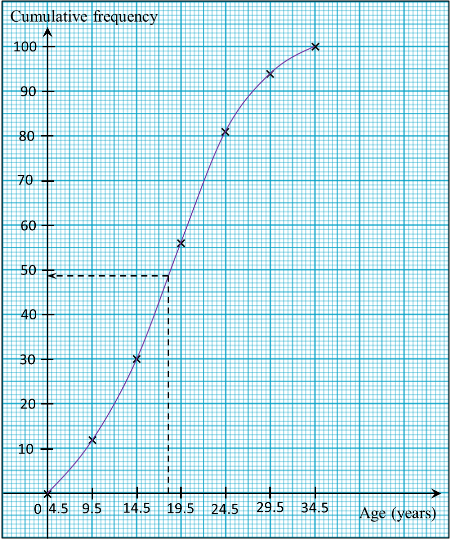
(c)

(d)
Third quartile
= 75th student
= 90.0 kg
Diagram shows a histogram which represents the mass, in kg, for a group of 100 students.
Diagram(a) Based on the Diagram, complete the Table in the answer space.
(b) Calculate the estimated mean mass of a student.
(c) For this part of the question, use graph paper. You may use a flexible curve ruler.
Using a scale of 2 cm to 10 kg on the horizontal axis and 2 cm to 10 students on the vertical axis, draw an ogive for the data.
(d) Based on the ogive drawn in 10(c), state the third quartile.
Answer:
Solution:
(a)
(b)
(c)
(d)
Third quartile
= 75th student
= 90.0 kg
 Diagram


 Diagram
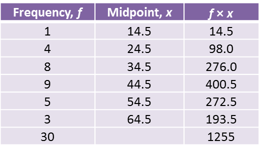
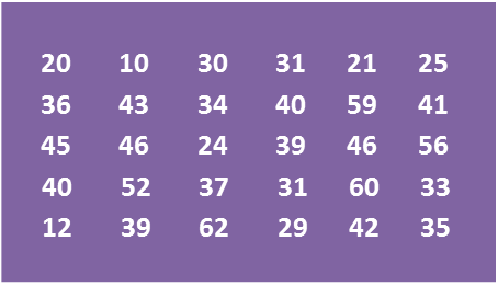
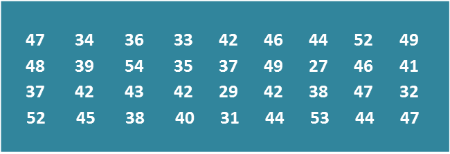
 Table
Table

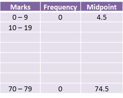
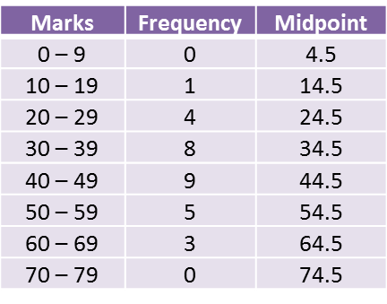
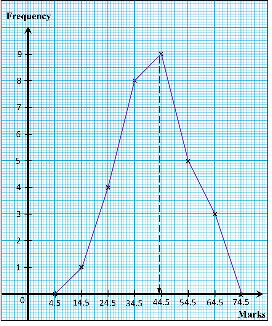
 (a) Using data in diagram above and a class interval of 5 marks, complete the table in the answer space.