[adinserter block="3"]
[adinserter block="3"]
9.9 Small Changes and Approximations
,

,
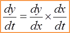
This is very useful information in determining an approximation of the change in one variable given the small change in the second variable.
[adinserter block="3"]
Example:
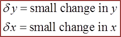
The small change in y is denoted by δy while the small change in the second quantity that can be seen in the question is the x and is denoted by δx.
Given that y = 3x2 + 2x – 4. Use differentiation to find the small change in y when x increases from 2 to 2.02.
Solution:
The small change in y is denoted by δy while the small change in the second quantity that can be seen in the question is the x and is denoted by δx.


 It is given that OP = 17 cm and PQ = 8.8 cm.