1. The scientific method is a systematic method in doing their work.
2. A report of the investigation must include:
   1. Objective of the experiment,
   2. Inference,
   3. Hypothesis,
   4. Three types of variables: manipulated variable, responding variable and fixed variable,
   5. Defined operational variables,
   6. List of apparatus,
   7. Procedure,
   8. Tabulation of data,
   9. Analysis of data,
   10. Conclusion

Inference:

Inference is a statement to state the relationship between two visible quantities observed in a diagram or picture.

Hypothesis:

Hypothesis is a statement to state the relationship between two measurable variables that can be investigated in a lab.

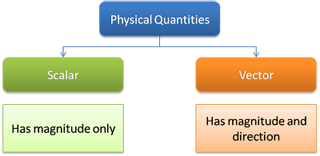
Variables.

A variable is a quantity that can vary in value. There are 3 types of variable:

1. Manipulated Variables: Manipulated variables are factors which changed for the experiment.
2. Responding Variables: Responding variables are factors which depend on the manipulated variables.
3. Constant Variables: Constant variables are factors which are kept the same throughout the experiment.

Tabulating Data

A proper way of tabulating data should include the following:

1. The name or the symbols of the variables must be labelled with respective units.
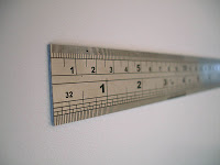
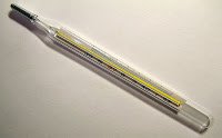
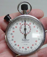
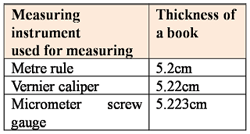
2. All measurements must be consistent with the sensitivity of the instruments used.
3. All the values must be consistent to the same number of decimal places.

Graph

Graphs are used to make a relationship between variables.
Gradient value and extrapolation of a graph are used to analyse a graph.
A well-plotted must contain the following features:

1. A title to show the two variables under investigation,
2. two axes labelled with the correct variables and their respective units,
3. the graph drawn is greater than 50 % of the graph paper,
4. appropriate scales (1:1 x 10^x, 1:2 x 10^x and 1:5 x 10^x)
5. all the points are correctly plotted,
6. a best fit line is drawn

1. Ammeters are measuring instrument used to measure electric current.
2. Voltmeters are measuring instrument used to measure potential difference (voltage).
3. In SPM syllabus, you need to know
   1. how to take reading from ammeter and voltmeter
   2. how to identify the sensitivity of an ammeter and voltmeter.
   3. the connection of ammeter and voltmeter in a circuit.
4. An ammeter is always connected in series with the load (resistor) in a circuit.
5. A voltmeter is always connected parallel to the load (resistor) in a circuit.

Label of the Parts

Range and Accuracy

1. The range of a micrometer is 0-25mm.
2. The accuracy of a micrometer is up to 0.01mm.

How to Use a Micrometer?

1. Turn the thimble until the object is gripped gently between the anvil and spindle. 
2. Turn the ratchet knob until a "click" sound is heard. This is to prevent exerting too much pressure on the object measured. 
3. Take the reading.

How to Read the Reading?

Reading = Reading of main scale + Reading of thimble scale.

Reading of main scale = 0 - 25 mm
Reading of thimble scale = 0 - 0.49mm

Example

(This image is licensed under GDFL. The source file can be obtained from wikipedia.org.)

Reading of main scale = 5.5mm
Reading of thimble scale = 0.28mm

Actual Reading = 5.5mm + 0.28mm = 5.78mm

Precaution Steps

1. The spindle and anvil are cleaned with a tissue or cloth, so that any dirt present will not be measured. 
2. The thimble must be tightened until the first click is heard. 
3. The zero error is recorded.

1. Vernier caliper is a measuring tool used to measure length.
2. It is more accurate than metre rule. It can measure length with an accuracy up to 0.01cm.
3. Figure above shows the illustration of a vernier caliper. For SPM students, you need to remember the name aof the parts and the function of the 2 jaws and the stem.

Taking Reading from a Vernier Calipers:

Zero Error of Vernier Caliper

1. The zero error is determined by tightening the jaws of the vernier calipers.
2. Zero error must be eliminated from the reading.

Ruler

1. Make sure that the object is in contact with the ruler.
2. Avoid parallax error.
3. Avoid zero error and end error.

Thermometer

1. Thermometers of range -10°C - 110°C with accuracy 1°C.
2. Thermometers of range 0°C - 360°C with accuracy 2°C.

1. Make sure that the temperature measured does not exceed the measuring range.
2. When measuring temperature of liquid.
   1. immerse the bulb fully in the liquid
   2. stir the liquid so that the temperature in the liquid is uniform
   3. do not stir the liquid vigorously to avoid breaking the thermometer

Stopwatch

(The image is licienced under GDFL. The source file can be obtained at wikipedia.org.)

1. analogue stopwatches of sensitivity 0.1s or 0.2s
2. digital stopwatches of sensitivity 0.01s.

Consistency

1. Consistency (or precision) is the ability of an instrument in measuring a quantity in a consistent manner with only a small relative deviation between readings.
2. The consistency of a reading can be indicated by its relative deviation.
3. The relative deviation is the percentage of mean deviation for a set of measurements and it is defined by the following formula:

Accuracy

1. The accuracy of a measurement is the approximation of the measurement to the actual value for a certain quantity of Physics.
2. The measurement is more accurate if its number of significant figures increases.
3. Table above shows that the micrometer screw gauge is more accurate than the other measuring instruments.
   
4. The accuracy of a measurement can be increased by
   1. taking a number of repeat readings to calculate the mean value of the reading. 
   2. avoiding the end errors or zero errors. 
   3. taking into account the zero and parallax errors. 
   4. using more sensitive equipment such as a vernier caliper to replace a ruler. 
5. The difference between precision and accuracy can be shown by the spread of shooting of a target (as shown in Diagram below).

Sensitivity

1. The sensitivity of an instrument is its ability to detect small changes in the quantity that is being measured.
2. Thus, a sensitive instrument can quickly detect a small change in measurement.
3. Measuring instruments that have smaller scale parts are more sensitive.
4. Sensitive instruments need not necessarily be accurate.

1. Error is the difference between the actual value of a quantity and the value obtained in measurement.
2. There are 2 main types of error 
   1. Systematic Error 
   2. Random Error

Systematic Error

1. Systematic errors are errors which tend to shift all measurements in a systematic way so their mean value is displaced. Systematic errors can be compensated if the errors are known.
2. Examples of systematic errors are
   1. zero error, which cause by an incorrect position of the zero point, 
   2. an incorrect calibration of the measuring instrument. 
   3. consistently improper use of equipment. 
3. Systematic error can be reduced by
   1. Conducting the experiment with care.
   2. Repeating the experiment by using different instruments.
      

Zero error

1. A zero error arises when the measuring instrument does not start from exactly zero.
2. Zero errors are consistently present in every reading of a measurement.
3. The zero error can be positive or negative.

(NO ZERO ERROR: The pointer of the ammeter place on zero when no current flow through it.)

Random errors

1. Random errors arise from unknown and unpredictable variations in condition.
2. It fluctuates from one measurement to the next.
3. Random errors are caused by factors that are beyond the control of the observers.
4. Random error can cause by
   1. personal errors such as human limitations of sight and touch. 
   2. lack of sensitivity of the instrument: the instrument fail to respond to the small change. 
   3. natural errors such as changes in temperature or wind, while the experiment is in progress. 
   4. wrong technique of measurement. 
5. One example of random error is the parallax error. Random error can be reduced by 
   1. taking repeat readings 
   2. find the average value of the reading.

Parallax error

A parallax error is an error in reading an instrument due to the eye of the observer and pointer are not in a line perpendicular to the plane of the scale.

Prefixes are the preceding factor used to represent very small and very large physical quantities in SI units.

Table below shows the prefixes that you need to know in SPM.

Conversion of prefixes

Prefixes to Normal Number

Normal number to Prefixes

1. Scientific notation (also known as Standard index notation) is a convenient way to write very small or large numbers. 
2. In this notation, numbers are separated into two parts, a real number with an absolute value between 1 and 10 and an order of magnitude value written as a power of 10.

Significant Figure

1. In measurement, significant figures relate the certainty of the measurement.
2. As the number of significant figures increases, the certainty of the measurement increase, which means we are more certain about what we have measured.

Scalar Quantity

1. Scalars are quantities which are fully described by a magnitude alone. 
2. Magnitude is the numerical value of a quantity. 
3. Examples of scalar quantities are distance, speed, mass, volume, temperature, density and energy. 

Vector Quantity

1. Vectors are quantities which are fully described by both a magnitude and a direction. 
2. Examples of vector quantities are displacement, velocity, acceleration, force, momentum, and magnetic field.